Thinking alternatively - Part two
In ‘An introduction to alternatives investing’ we defined alternatives as investments that deliver uncorrelated returns. The terms 'uncorrelated returns' and 'diversification' are related and are a common objective when constructing investment portfolios. Understanding what those terms really mean is essential to properly appreciate how alternative investments can contribute to robust long-term portfolios.
This second piece in our ‘Thinking alternatively’ series examines correlation and the diversification benefits delivered by low correlation in more detail. We explore the nature of correlation and how the inclusion of uncorrelated assets in investment portfolios can lead to more robust returns and enhance outcomes through the power of diversification. We demonstrate how seemingly minor changes in correlation between assets can have a significant impact on overall portfolio performance. We also highlight the potential challenges when determining the correlation between assets and the key factors investors should consider to maximise the benefits of uncorrelated investments.
What is correlation?
Correlation is a statistical measure of the relationship between the returns (rather than price levels) of two different investments. Correlation can range between -1 and +1. Investments that have high correlation can be viewed as moving in the same direction at the same time while those with little or no correlation move independently of each other. Negatively correlated investments tend to move in opposite directions.
Importantly, two investments that both deliver positive returns over longer periods can nevertheless exhibit zero or even negative correlation. Similarly, two investments that move in opposite directions over time can nevertheless be positively correlated. For example, the daily price moves of an investment may show a very different relationship than the point-to-point one-year return.
In figure 1, as an illustration, at first glance it may appear that the two investments shown in the left-hand chart below are positively correlated. After all, for the period shown, both have increased by about the same amount. Looking at the daily returns in the chart on the right, we can see that most days the two investments do indeed move up together, however, on some days they move in opposite directions. Counterintuitively, the correlation of these two strategies turns out to be zero. An important implication is that investors can derive diversification benefits from two investments that both go up over time.
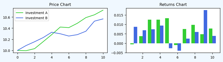
Figure 1: Low correlation is sometimes hard to spot. Investment A and B look like they’re similar, however correlation is zero.
It’s also important to note that statistically high correlation does not imply causation. The observation that the two return series are highly correlated does not (necessarily) imply that the returns from investment X are positive because the returns from investment Y are positive.
Since correlation is not causation, it means correlation can change over time. When building portfolios, we therefore need to consider what factors might cause correlations to change, and under what circumstances that might occur.
Correlation also ignores the magnitude of the moves causing the relationship. Two investments that have very high correlation might move up and down by the same amount at the same time, or by very different amounts. Correlation captures the fact that they move up and down at the same time, not how much each moves up and down.
In summary:
- Correlation measures the relationship between the returns of two investments.
- Two investments that move in the same direction over time can be uncorrelated and two investments that move in opposite directions over time can be positively correlated.
- Correlation can change over time.
- Correlation can’t tell us how much one investment will move for a given move in another.
Why does it matter?
Simply put, by combining uncorrelated investments, we can construct portfolios with lower risk and/or higher returns. This is the power of diversification. The lower the correlation, the bigger the potential benefit. This is where alternatives come in - no other asset class offers the same variety and breadth of uncorrelated investments as the universe of alternative investments.
We illustrated how adding alternatives to a 60/40 balanced portfolio can both increase portfolio returns and decrease portfolio risk in ‘An introduction to alternatives investing’ and have reproduced the chart below. More generally, a good framework for assessing the benefits from diversification is the Markowitz Efficient Frontier1. This shows the combination of investments (i.e. portfolio) which gives the highest expected return for a given level of risk. By including additional investments, we can improve a portfolio’s position on the risk/return spectrum. The chart on the right shows the efficient frontier for a base portfolio of cash, global fixed income and global equities before and after the introduction of alternatives. The green line is above the blue one, demonstrating that by including alternatives, investors can achieve higher portfolio returns for any given level of risk.
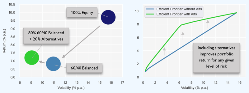
Figure 2: The efficient frontier shows the optimal portfolio (the one giving the highest expected return) for any given level of risk. Including uncorrelated positive expected return investments such as alternatives improves the efficient frontier, indicating the possibility of enhancing portfolio returns. Historical returns are calculated using quarterly data from December 2013 until December 2021. Equity is MSCI ACWI Net Total Return USD, Fixed Income is Bloomberg Global Aggregate USD, Cash is Fed Funds Total Return and Alternatives is an equally weighted portfolio of Bloomberg All Hedge Fund, Bloomberg Buyout Private Equity and Bloomberg Real Asset Private Equity.
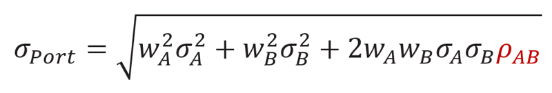
To see why uncorrelated assets, produce better portfolios, consider two separate investments A and B, both with an expected return of 10% p.a. and a volatility of 10%. The volatility of the portfolio of A and B can be expressed mathematically as 2:
Portfolio volatility is directional with correlation, i.e. higher correlation leads to higher portfolio volatility. Figure 3 below shows how different levels of correlation between A and B result in very different outcomes when combining A and B into an equally weighted portfolio.
| Expected return A | 10% |
| Expected return B | 10% |
| Volatility A | 10% |
| Volatility B | 10% |
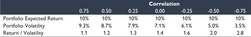
Figure 3: Diversification illustration for a simple portfolio of two assets
Observe what happens to the portfolio volatility when correlation is low or even negative. As correlation decreases so too does portfolio volatility, to levels far below that of either A or B individually. Risk-adjusted returns for the portfolio therefore improve substantially (same return with lower risk) as correlation decreases.
We can expand the concept for a larger portfolio. We take 50 completely uncorrelated (i.e. correlation=0) investments, all with the same ex-ante expected return and ex-ante volatility, and a modestly positive Sharpe Ratio3 of 0.3. However, investing in an equally weighted portfolio of those same investments results in the green line in the left-hand chart. The Sharpe Ratio of the portfolio is 1.94, a significant improvement on any individual investment.
Now, let’s consider the case when the pair-wise correlation of the underlying investments is +0.25. Although the underlying investments still have quite low correlation to each other, the cumulative portfolio return in this instance is dramatically lower than when correlation was zero, shown by the blue line in the right-hand chart. The portfolio’s Sharpe Ratio has dropped to 0.57. While still an improvement on the underlying investments, the diversification benefit has been diluted substantially by only a modest increase in correlation.
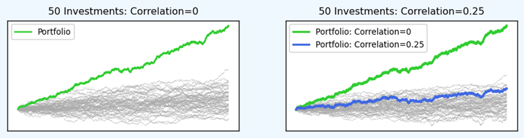
Figure 4: Cumulative returns for portfolios of (un)correlated investments. Underlying investments are simulated assuming a Sharpe Ratio of 0.3 and pair-wise correlation of either 0 or +0.25. Portfolio returns are volatility scaled to match the underlying investments.
The above is, of course, a contrived example from a simulation. However, it illustrates just how powerful the combination of uncorrelated investments can be. This is where alternatives have the potential to play such an important role in investment portfolios.
Back in the real world, it is difficult, if not impossible, to find the 50 truly uncorrelated investments that produce the green line in the chart above. Nevertheless, every additional uncorrelated investment introduced into a portfolio increases the potential diversification benefits for the portfolio. Since alternative investments are often uncorrelated to each other as well as to traditional asset classes, they are a rich hunting ground for investors seeking to maximise the power of diversification.
There is, unfortunately, an important caveat. Just as low (or even better negative) correlation can result in powerful diversification benefits, even relatively small changes in the correlations between portfolio components have the potential to reduce the diversification benefit. Observe the difference between the green and blue lines in the right-hand chart above.
What factors affect correlation?
Geopolitical events, economic cycles and risk off periods are just some of the factors that can lead to changes in correlation. This is important, because changes in correlation can lead to the loss of diversification benefits, potentially undermining portfolio performance.
Extreme market events such as COVID during March 2020 can cause sharp increases in correlation. Even if only temporary, this can have a devastating impact on portfolios if previously uncorrelated investments all move in the same direction (usually down) at the same time.
The change in correlation between bonds and equities in 2022 was another stark reminder of how changes in correlation can negatively impact portfolio returns. Any investor who assumed fixed income would provide a defensive buffer against a drawdown in equities was sorely disappointed last year, with the traditional 60/40 balanced portfolio delivering -21.7% 4. In this instance, the rapid increase in interest rates was the cause of the re-rating of equity markets and returns from both equities and fixed income were negative. Correlation isn’t causation, but causation is, by definition, correlation.
Understanding where there might be common factors driving the returns of two different investments is therefore essential when thinking about how correlation might change. In 2022, higher interest rates negatively impacted performance for many different investments, some alternatives included. For example, bonds, equities, real estate, private equity and digital assets all sold off together – higher interest rates caused correlation to increase meaning investors suffered simultaneous negative returns in those assets.
Investors who anticipate changes in market environment that could impact correlations may be able to maintain diversification by rebalancing away from investments susceptible to a change in correlation and toward investments that aren’t. However, this can be difficult, so seeking alternative investments that are less susceptible to correlation changes to serve as 'anchor' diversifiers in a portfolio can be a useful strategy. This can be part of a broader alternatives investing approach, whereby different alternative investments play different roles in the portfolio.
What are the challenges with correlation?
Investors who can successfully source uncorrelated alternative investments will be able to build more robust investment portfolios with more consistent returns through the power of diversification. On paper, all uncorrelated investments will provide diversification benefits. However, as outlined above, investors need to exercise caution when measuring correlation and assessing the suitability of any investment. For starters, there is no single measure of historical correlation investors can use to determine 'true' correlation.
Questions to consider include:
- What historical period should be used: measured daily, weekly, monthly or even quarterly?
- How stable is correlation over time? Is the measured correlation low, but when looking at rolling correlations there are periods of very high correlations offset by periods of very low or even negative correlation?
- When, and under what circumstances is correlation high? Do periods of high correlation coincide with periods of stress in other parts of the portfolio, in which case an investor might be losing diversification benefits when they need them most?
All these questions, and more, need to be addressed. Some simple things investors can consider when analysing correlation include:
- Calculate rolling correlation over shorter periods and observe how correlation changes over time. No two investments will have perfectly stable correlation at all points in time, but equally, an investment that has very negative correlation at some times and very positive correlation in others might not provide the long-term diversification benefits investors are looking for. This might also help identify any patterns in correlation that can be further investigated.
- Calculate conditional correlations. For example, calculate correlation using only data points where equity returns are negative. If equities are a core part of the portfolio, investments which have low correlation looking at all data, but high correlation when equities are performing badly may not turn out to be as diversifying as an investor might like in the circumstances when diversification is needed most. Depending on the investment objective, different conditioning rules may be more or less appropriate.
- Account for regime changes. Has some exogenous change resulted in a fundamental change in the relationship between two investments? Investors can attempt to model such changes, or at a minimum monitor correlation to check nothing has meaningfully changed.
- Remember that correlation is only one aspect of what makes a potential investment attractive. Risk/return profiles of different investments might be attractive even where there is higher correlation to existing portfolio components. For example – as we discussed in An introduction to alternatives investing – alternatives can be used to reshape portfolio return distributions in ways that might be desirable to investors even in the absence of large diversification benefits. For example, alternatives might provide higher returns and/or lower volatility regardless of correlation.
The more confidence an investor has that they understand the broad correlation characteristics of an investment, the more confidence they can have around the diversification benefits they can unlock by including that investment in their portfolio.
Final thoughts
Correlation measures the relationship between returns from different investments. As with many financial variables, measuring correlation is not quite as straightforward as it might at first appear. Importantly, correlation is estimated using historical movements, however, because correlation and causation are different, there is no guarantee that correlation won’t change in the future.
Once we have estimates of correlation (along with risk and returns) for a set of investments, we can measure the diversification benefit. Returns will be higher for any given level of risk for combinations of investments with low correlation than for combinations with high correlation. As a concept, correlation can therefore be an essential part of assessing any potential investment and is of particular importance when considering alternative investments.
A solid understanding of correlation, its applications and limitations allows investors to unlock the power of diversification. Alternatives tend to be uncorrelated to other asset classes and can therefore be an excellent source of diversification. Correlations can change, however, so alternative investments which deliver consistently low correlation to traditional assets can be particularly valuable in building robust, resilient portfolios.
1 Markowitz, H.M. (March 1952). “Portfolio Selection”. The Journal of Finance.
2 σ2 is the volatility of asset i, wi is the weight of i in the portfolio, and 𝑝j is the correlation of i and j.
3 The Sharpe Ratio is a commonly used metric which is calculated as the ratio of the excess return to the volatility of an investment. It can be interpreted as a measure of the return per unit of risk.
4 Calculated using 60% MSCI World (AUD Hedged) and 40% Bloomberg Global Aggregate (AUD Hedged) rebalanced daily.
This material has been prepared by Challenger Investment Solutions Management Pty Ltd (ABN 63 130 035 353, AFSL 487354) (CISM) for wholesale investors only. The information in this material is general information only and is not intended to be financial product advice. It has been prepared without taking account of any person’s objectives, financial situation or needs. The information in this material has not been independently verified. No reliance may be placed for any purpose on the material for its accuracy, fairness, correctness or completeness. To the extent permitted by law, no liability is accepted for any loss or damage as a result of reliance on this information.
Related content
.png?h=325&iar=0&w=500)
Different alternatives achieve different things
.png?h=325&iar=0&w=500)